Introduction
Sequential control is one of the most common requirements in industrial automation. Whether you are starting a pump sequence, managing a conveyor cycle, or coordinating a multi-step process, you need logic that does not just react to the current state of inputs but also tracks what has already happened. A sensor reading TRUE means something different depending on whether the machine just started or has been running for five seconds.
The standard approach many reach for is a combination of timer-driven sequencers, one-shots stitched together with retentive bits, or a pile of interlocks that grow increasingly hard to follow with every revision. These approaches work, but they tend to produce code that is difficult to read, harder to document, and painful to modify.
A better approach is to model the problem as a Finite State Machine (FSM) from the start, and then translate that model directly into ladder logic in a structured, repeatable way. This post walks through exactly that process, using a simple conveyor system as the example. By the end you will have a reusable pattern you can apply to any sequential control problem in Studio 5000.
The methodology used here is based on a two-part technical series by Greg Schmidt published on control.com, titled State Machine Programming in Ladder Logic (November 2020) and Advanced Methods of State Machine Programming in Ladder Logic (November 2020). I have adapted and extended that methodology for Rockwell Studio 5000 specifically, incorporating lessons learned from applying it on real projects.
What Is a Finite State Machine?
A finite state machine is a model of sequential behavior built around two core concepts: states and transitions.
A state represents a distinct, stable condition that a piece of equipment or process can be in. At any given moment, the machine is in exactly one state. The state determines what actions are being taken and what inputs are being monitored.
A transition is a directed change from one state to another. Transitions are driven by events: conditions that become true while the machine is in a particular state. When an event fires, the machine leaves the current state, performs any entry actions associated with the new state, and begins monitoring for the events defined in the new state.
The power of this model is that it forces you to think through every combination of state and input explicitly. You cannot write code for an event without first deciding which state that event applies to. This discipline eliminates a large class of bugs that arise from inputs being handled in the wrong context.
For ladder logic, the FSM maps cleanly onto a structured routine organized into three sections, executed in order every scan:
- Events – Rungs that evaluate physical inputs and derive the event bits used by the rest of the routine.
- State Transitions – Rungs that check the current state, monitor for events, and update the state index when a transition fires.
- State Commands – Rungs that execute the actions associated with each state, typically on entry using a one-shot.
The Example: Conveyor CV1
The example we will implement is a simple conveyor system described in Schmidt’s original articles. It is deliberately straightforward so the focus stays on the methodology rather than the machinery.
Physical Description
The operator places a load at the far right end of the conveyor and presses the Start button. The conveyor motor runs, moving the load to the left. When the load reaches the left end, it blocks a photoeye. The conveyor stops and waits. An external module eventually sends an eject command, the conveyor runs again to transfer the load off, and once the photoeye clears, the conveyor returns to idle and is ready for the next cycle.
A Stop button allows the operator to halt the conveyor mid-cycle. A 10-second fault timer detects if the load fails to reach the photoeye within a reasonable time. If the timer expires, the conveyor stops and a fault is latched. An HMI button allows the operator to clear the fault and return to idle.
The physical I/O is minimal:
Start_PB– Start push-button (momentary NO)Stop_PB– Stop push-button (momentary NO)Photoeye– Photoeye input (1 = blocked, 0 = clear)CV1_C1– External eject command bit (set by another module)CV1_Motor– Conveyor motor run command outputHMI_FaultClear– HMI momentary button for fault reset
State Transition Diagram
Before writing a single rung of ladder logic, define the FSM on paper. The diagram below shows all five states and the events that drive transitions between them.
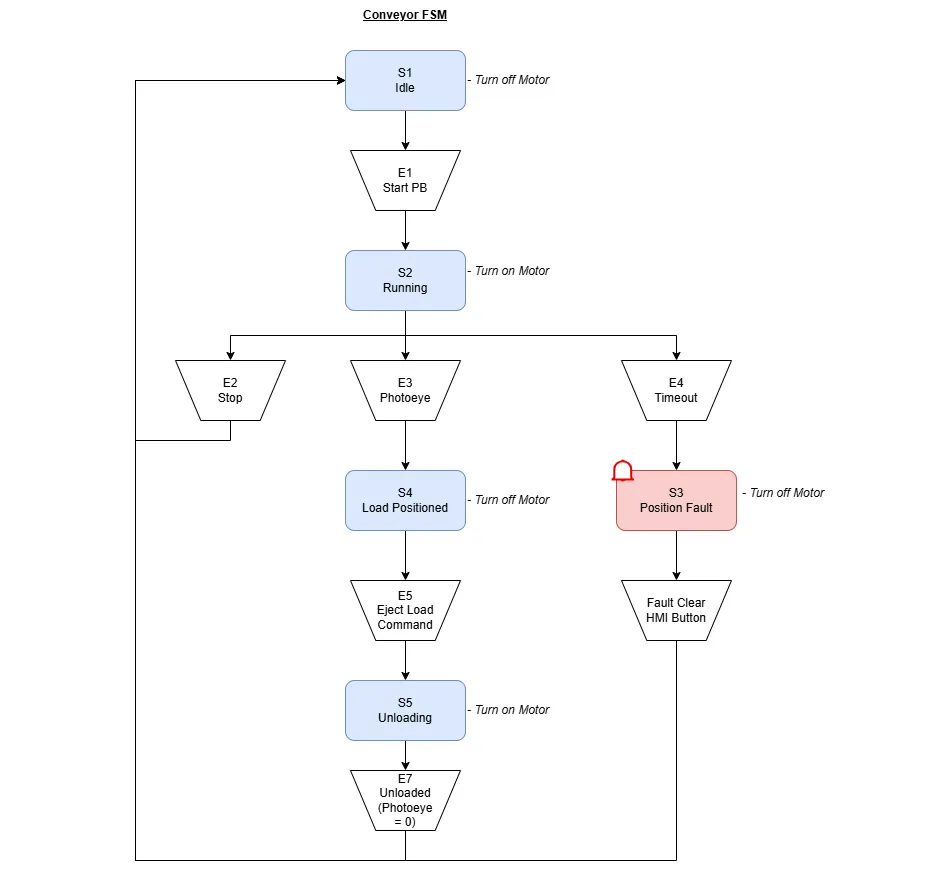
The five states are:
| Index | State Name | Description |
|---|---|---|
| 1 | S1 – Idle | Conveyor stopped, waiting for operator to load and press Start |
| 2 | S2 – Running | Motor on, load traveling toward photoeye, fault timer accumulating |
| 3 | S3 – Position Fault | Motor off, fault latched, waiting for operator to clear via HMI |
| 4 | S4 – Load Positioned | Motor off, load at photoeye, waiting for external eject command |
| 5 | S5 – Unloading | Motor on, load being transferred off conveyor |
The seven events are:
| Tag | Event | Set When |
|---|---|---|
| E1 | Start | Start_PB pressed |
| E2 | Stop | Stop_PB pressed |
| E3 | Load Positioned | Photoeye blocked |
| E4 | Position Timeout | CV1_Timer.DN (latched) |
| E5 | Eject Load Command | CV1_C1 set by external module |
| E7 | Load Ejected | Photoeye cleared (XIO) |
Note that E6 is intentionally absent from this implementation. The eject complete handshake originally assigned to E6 was left out to simplify this example.
Module Documentation
Good FSM practice requires documenting the full transition table before touching Studio 5000. The table below is the formal specification for CV1. Every row in the State Transitions section of the ladder logic corresponds directly to one row of this table.
| Current State | Event | Next State | Notes |
|---|---|---|---|
| S1 Idle | E1 – Start | S2 Running | |
| S2 Running | E2 – Stop | S1 Idle | Operator halt |
| S2 Running | E3 – Load Positioned | S4 Load Positioned | Normal completion |
| S2 Running | E4 – Position Timeout | S3 Position Fault | Fault condition |
| S3 Position Fault | HMI_FaultClear | S1 Idle | Requires operator action |
| S4 Load Positioned | E5 – Eject Load Command | S5 Unloading | External command |
| S5 Unloading | E7 – Load Ejected | S1 Idle | Photoeye clears |
Implementation in Studio 5000
Tag Structure
The FSM uses a small set of dedicated tags. All are program-scoped.
State Index (CV1_FSM_Idx, DINT): Holds the current state number. The value should be initialized to 1 (S1 Idle) so the conveyor starts in a known state on first download.
One-Shot Bit (CV1_FSM_ONS, BOOL): This is the key to how the FSM manages transitions. It starts initialized to 1 (TRUE). Each transition rung uses ONS(CV1_FSM_ONS) as a condition. When a transition fires, the rung immediately unlatches it with OTU(CV1_FSM_ONS). Because the ONS bit is now FALSE, no other transition rung can fire on the same scan. The bit stays FALSE until the next scan begins, at which point the ONS() instruction in the new state’s transition rung will see it as TRUE again and allow normal evaluation. This guarantees exactly one state change per scan.
OSR Pairs (S#_OSRs / S#_OSRo, BOOL): Each state gets a one-shot rising (OSR) instruction pair in the State Commands section. These detect entry into a state and allow actions to execute once on entry rather than every scan. The storage bit (OSRs) is what the OSR instruction writes to internally. The output bit (OSRo) goes TRUE for exactly one scan after the EQ condition becomes TRUE, i.e., the scan immediately after entering the state.
Fault Timer (CV1_Timer, TIMER): A standard TON with a 10-second preset. Placed inside the S2 transition rung so its accumulation and reset are managed in one place.
Event Bits (E1-E5, E7, BOOL): Intermediate bits derived from physical inputs in the Events section. Decoupling the physical input from the event bit makes the transition logic cleaner and allows the same physical input to drive multiple events (as Photoeye does for both E3 and E7).
Alarm Bit (S3_Alarm, BOOL): A latched bit that holds the fault condition. Latched with OTL when E4 fires during the S2 transition. Cleared with OTU when the operator successfully resets from S3.
Section 1: Events
The Events section is a set of straightforward output rungs. Each rung evaluates a physical input and drives an event bit.
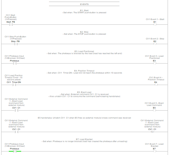
XIC(Start_PB)OTE(E1);
XIC(Stop_PB)OTE(E2);
XIC(Photoeye)OTE(E3);
XIC(CV1_Timer.DN)OTE(E4);
XIC(CV1_C1)OTE(E5);
XIC(CV1_C1)OTU(CV1_C1);
XIO(Photoeye)OTE(E7); E7 uses XIO(Photoeye) rather than XIC. The photoeye is blocked (TRUE) when the load is present and clear (FALSE) when the load has exited. E7 is the “load ejected” event, which means it should fire on the falling edge of the photoeye, i.e., when the photoeye transitions from blocked to clear.
The E5 handshake on Rung 6 deserves a mention. When the external module sets CV1_C1 to command an eject, this routine immediately unlatches it. This acts as a consumed-command handshake: the external module can check that C1 has gone back to FALSE to confirm the command was received.
Section 2: State Transitions
The State Transitions section is the heart of the FSM. Each rung follows the same pattern:
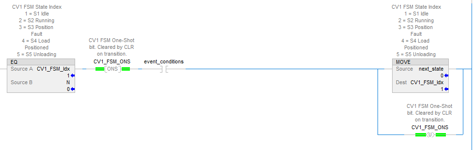
Breaking this down:
EQ(CV1_FSM_Idx, N)– This rung only evaluates when the current state index equals N.ONS(CV1_FSM_ONS)– Ensures only one transition can fire per scan.[event conditions]– XIC on one or more event bits.MOVE(next_state, CV1_FSM_Idx)– Updates the state index to the new state.OTU(CV1_FSM_ONS)– Clears the ONS bit so no further transitions fire this scan.
When a state has multiple possible transitions, parallel branches are used inside a single rung. Each branch independently checks its event and executes its own MOVE and OTU if the event is TRUE.
S1: Idle
S1 has only one exit path: E1 (Start PB). When E1 is TRUE, the index moves to 2 (Running) and the ONS bit clears.
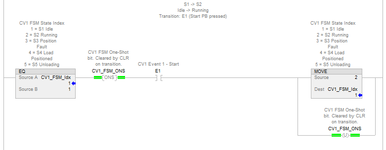
EQ(CV1_FSM_Idx,1)ONS(CV1_FSM_ONS)XIC(E1)[MOVE(2,CV1_FSM_Idx),OTU(CV1_FSM_ONS)]; S2: Running
This is the most complex rung in the routine and illustrates two important aspects of the implementation.
First, the three parallel branches handle the three possible exits from S2. If E4 fires, the S3_Alarm bit is latched in addition to the state change to S3.
Second, the RES(CV1_Timer) and TON(CV1_Timer,?,?) instructions are appended after the parallel branch group, in series with the EQ and ONS conditions. This means:
- While in S2 with no active transition, the rung evaluates TRUE through EQ and ONS, skips over any branch (none of E2/E3/E4 are TRUE), and executes the TON, accumulating time.
- When a transition fires (any branch executes), the MOVE updates the state index. On the very same scan, the RES immediately resets the timer, ensuring a clean reset. On the next scan the EQ fails (we are no longer in state 2), so neither the timer nor any branch evaluates again until the machine returns to S2.
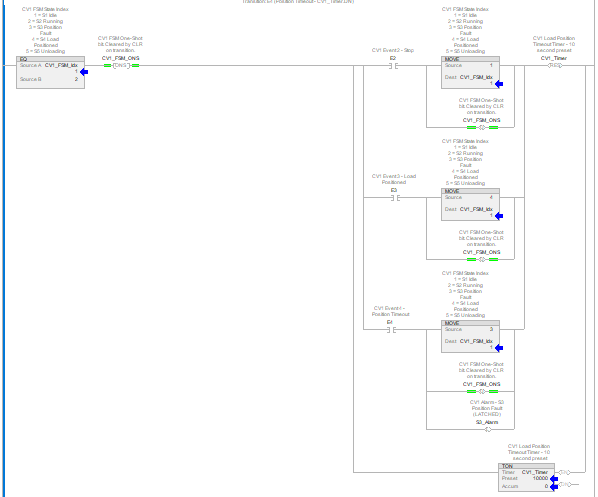
EQ(CV1_FSM_Idx,2)ONS(CV1_FSM_ONS)[[XIC(E2)[MOVE(1,CV1_FSM_Idx),OTU(CV1_FSM_ONS)],XIC(E3)[MOVE(4,CV1_FSM_Idx),OTU(CV1_FSM_ONS)],XIC(E4)[MOVE(3,CV1_FSM_Idx),OTU(CV1_FSM_ONS),OTL(S3_Alarm)]]RES(CV1_Timer),TON(CV1_Timer,?,?)]; S3: Position Fault
S3 waits for the operator to press the HMI fault clear button. When they do, two things happen: the state returns to S1 and the alarm bit is cleared.
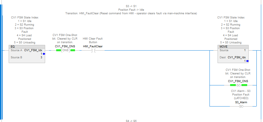
EQ(CV1_FSM_Idx,3)ONS(CV1_FSM_ONS)XIC(HMI_FaultClear)[MOVE(1,CV1_FSM_Idx),OTU(CV1_FSM_ONS),OTU(S3_Alarm)]; S4: Load Positioned
S4 waits for the external eject command. One exit path, clean and simple.
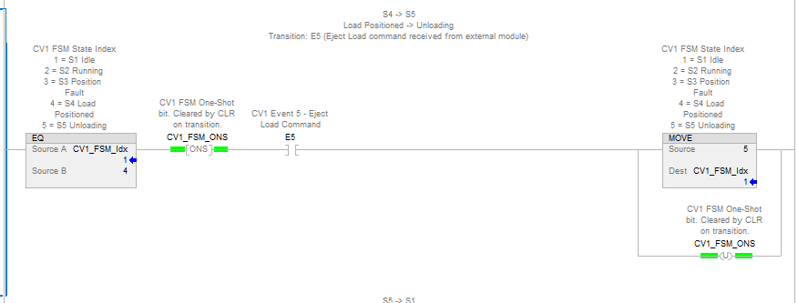
EQ(CV1_FSM_Idx,4)ONS(CV1_FSM_ONS)XIC(E5)[MOVE(5,CV1_FSM_Idx),OTU(CV1_FSM_ONS)]; S5: Unloading
S5 waits for the photoeye to clear, confirming the load has fully exited the conveyor. When it does, the machine returns to S1 Idle and the cycle can begin again.
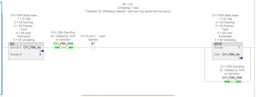
EQ(CV1_FSM_Idx,5)ONS(CV1_FSM_ONS)XIC(E7)[MOVE(1,CV1_FSM_Idx),OTU(CV1_FSM_ONS)]; Section 3: State Commands
The State Commands section handles the actions associated with each state. The pattern for every state is two rungs: an OSR detection rung and an action rung.
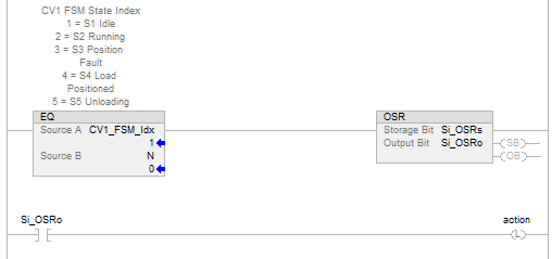
The OSR() instruction monitors the EQ condition. On the first scan that the EQ is TRUE (meaning the state was just entered), Si_OSRo goes TRUE for exactly one scan. The action rung fires once on entry and does not repeat unless the state is exited and re-entered.
The entry actions for each state are:
| State | Entry Actions |
|---|---|
| S1 – Idle | OTU(CV1_Motor) – Turn motor off |
| S2 – Running | OTL(CV1_Motor) – Turn motor on |
| S3 – Position Fault | OTU(CV1_Motor) – Turn motor off |
| S4 – Load Positioned | OTU(CV1_Motor) – Turn motor off |
| S5 – Unloading | OTL(CV1_Motor) – Turn motor on |
The motor uses OTL/OTU (retentive latch/unlatch) rather than OTE (non-retentive output) because multiple states share the same output and the OSR pattern only drives it for one scan. OTE would drop the output immediately after the first scan. The retentive instructions ensure the motor state holds until explicitly changed and avoids issues that arise from destructive references.
Key Design Principles and Takeaways
Having walked through the full implementation, a few principles stand out as worth carrying into any FSM-based ladder logic project.
One state at a time, guaranteed. The CV1_FSM_Idx DINT combined with the ONS(CV1_FSM_ONS) / OTU(CV1_FSM_ONS) pattern ensures the machine is always in exactly one state and can only change state once per scan. This is structurally enforced, not dependent on programmer discipline.
Timers belong in the transition section. When a timer drives a state exit, placing the TON and RES in the transition rung tightly couples the timer’s lifecycle to the state’s lifecycle. The timer starts when you enter the state (EQ becomes TRUE), accumulates each scan, and resets atomically on the scan the transition fires. There is no risk of a stale accumulated value carrying over to the next entry.
Keep event derivation and transition logic separate. The Events section is a clean, readable record of what conditions mean in this process. A technician troubleshooting on the floor can look at the event bits in the Watch window and immediately understand what the machine sees, without parsing transition logic.
Document before you code. The state transition table in the Module Documentation section above is not just commentary for the blog post. In practice, that table is written before the ladder logic exists, and the ladder logic is a direct mechanical translation of it. Any transition that does not appear in the table does not appear in the ladder logic.
The FSM scales. The conveyor example has five states and seven events. A more complex machine might have fifteen states and twenty events. The structure does not change. Every state still gets one transition rung and two command rungs. The routine grows linearly and stays organized regardless of complexity.
Conclusion
The FSM methodology is not a new idea, but it is underused in industrial ladder logic. Most PLC programmers learn to write sequential logic by feel, accumulating experience with what works and what does not. The FSM approach replaces that trial-and-error with a structured design process: define states, define events, document the transition table, and translate it mechanically into ladder logic.
The Studio 5000 implementation shown here is a direct, faithful translation of that model. The three-section routine structure (Events, State Transitions, State Commands) maps one-to-one onto the three parts of the FSM definition. The state index, ONS bit, and OSR pairs are a small, reusable set of building blocks that can be dropped into any sequential control problem.
The L5X file for this implementation is available for download and can be imported directly into a Studio 5000 project as a starting point. All tags are declared with descriptions suitable for the Tag Editor. (If there are errors, simply upload the L5X file into your favorite LLM and ask it to adapt it to your version of Logix or fix any errors that arise in the Output window).
If this methodology finds its way into your next project, the payoff shows up at commissioning time, during troubleshooting, and especially the first time someone who did not write the code has to modify it six months later.
References:
- Greg Schmidt, “State Machine Programming in Ladder Logic,” Control.com, November 2020.
- Greg Schmidt, “Advanced Methods of State Machine Programming in Ladder Logic,” Control.com, November 2020.